
The financial domain is hugely complex and non-linear with a plethora of factors influencing each other.
Sonam Srivastava
Deep Learning has been the breakout approach to modelling and solving problems. It is currently, the SOTA (State of the Art) benchmarks for NLP and Computer Vision problems.
While, it has seen remarkable success, I yet to see very prominent output from using Deep Learning models especially RNN and very specifically LSTM based approaches, which seem best suited frameworks for this kind of time series modelling.
There has been a bunch of work written about using LSTMs and very toy example is a stock price prediction. But there are some inherent challenges in modelling capital markets data and how the output gets presented.
Data Challenges
- Non-Stationarity: In simple terms, the assumption of independence between data points is not valid unlike say a sequence of words. This gets solved by using either modelling returns or difference between data points.
- Insufficient Data: Unlike NLP and computer vision, the amount of data with a time series is limited. Even a 20-year history is not a lot of data points and oftentimes, the models will overfit and perform poorly out of sample.
- Data Regimes: Unlike CV and NLP, where the problem space is not dynamic in the sense that a CAT identified as one today, will continue to remain a CAT. Unless the data is obfuscated a lot.
- Markets are cyclical in nature and the testing part needs to represent that. The model needs to work across different regimes to be considered serious and robust.
- A model trained on bull phase will crack under bear or see-saw movements.
- Hedge funds and investment strategies have cracked when failing to deal with the scenario.
Research Challenges
- Survivorship Bias: There are countless prices and time series and you could have applied your approach to model any number of them and chosen the subset which represents the output you wanted to project.
- No standard datasets: Both NLP and CV have standard datasets over which any improvement in architecture is presented. This ensures parity in problem space and makes any comparison apples vs apples.
- Non-collaborative: Unlike tech, modelling for financial markets is closed room work. The exploits are used to make money than share. Rather deployed by firms for making money.
But, we had to carry out such a project, how would one go about it and what would be the key things to keep in mind. We definitely would be relying on the RNN class of learning because it’s the most attuned to this.
Key Aspects
There are couple of things to keep in mind when building these models:
- A naive baseline: This could be something as simple as last 20 days moving average as the predictor. This very simple baseline can be very difficult to beat or better.
- A domain baseline: This could be a domain-based line model which uses some probable features. This has to beat the naive baseline to be considered useful. Likely cases being ARIMA or linear models.
- Deep Learning Model: This model is now supposed to better both the domain and the naive baseline to be considered. Obviously, it would beat the naive model if domain beats the naive one.
- Time Horizon: What time horizon to predict for? Days, Months and Years? Makes little sense beyond months.
- Metric: The kind of metric to measure the error: MAPE and RMSE are the two obvious ones though RMSE is better due to the ability to punish extreme errors more significantly. MAPE is more intuitive for investment purposes.
ARIMA
Autoregressive integrated moving average should be one of the obvious ways of modelling time series problem and the basic construction of using the prediction (Y) as a function of previous values is also the basis for RNN based approaches.
Autoregressive means, we target the output variable on its past values.
Y = B0 + B1*Y_lag1 + B2*Y_lag2 ...The integrated part comes from the differencing step we undertake to make the data points stationary. This makes the equation more like
(Y1-Y0) = B0 + B1*(Y_lag1-Y_lag2) + B2*(Y_lag2-Y_lag3) ...The moving average part comes from regressing the outputs on the errors from the training set to adjust the values. This further improves the quality of the model.
This in short is the ARIMA model. When we use an RNN, we are using similar inputs and outputs if using an auto-regressive and no features but the relationship is non-linear and a lot more complex structure.
RNN (Different Deep Learning Architectures)
RNNs are Neural Network architectures designed keeping sequential data in mind. They also have multiple types of architectures depending on our needs. This is an awesome image of all types:
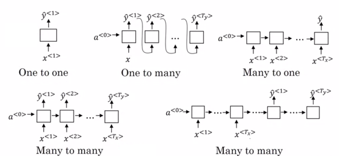
We might be interested in one-one and many-one type of problems in our context.
We had to build a model similar to the ARIMA discussed above, we would be using many to one architecture. Where the different inputs (x) are the inputs from different time steps for the model (Different instances of the same series by time)
There are broadly two types of outputs from each block in the model: a and y. Y being the output and a being the block outputs.

With the many-one architecture, we will have only one Y but many a’s. The activation functions are tanh and sigmoid. One of the key problems with this model is when processing the feedback from the error back to update the model.

These derivatives are used to update the model weights. Because of the sequences, progressive gradients typically either explode or get lost completely. This results in something called vanishing/exploding gradient problem.
To deal with the problem and ease the training part of the problem, LSTMs a special kind of RNNs are being used which use a more complex cell structure consisting of more number of gates which cap the gradient outputs and also act as filters.
LSTMs
Each cell of the RNN has multiple gates or activation functions serving a different purpose. The name Long-Short Term comes up the combination of these gates aka switches which preserve both long term memory and update short term feedback.

This is an awesome illustrative example of the exact working model about the LSTM model in the given pic and corresponding blog.
The forget gate helps train whether to keep the past information or not. The input gate acts a filter as of how much input information to pass through.
The remaining two are the output (hidden state) gates and the cell state inputs. These gates update the cell state and hidden state inputs. The combination of two kinds of outputs helps store or keep both long and short term thereby Long Short Term Memory model.
RNN have a single connection between the blocks and combined with vanishing/exploding gradient issue, this results in it having only short term memory and loses the ability to transfer long term memory.
For more classical machine learning-based use-cases in quantitative finance, check out this specific article.